IT Classics: A*
When teaching Artificial Intelligence (about 20 years ago), one of the topics I always covered was Pathfinding 1. Amongst many different techniques lies a very classical one: the A* (read "A star") 2.
The A* algorithm (introduced by Peter Hart, Nils Nilsson and Bertram Raphael 3) is a graph traversal and pathfinding algorithm that is used in many fields of computer science due to its completeness, optimality, and optimal efficiency 4. That means, given a graph, start and end nodes, the value for the weights, and the heuristic function, the A* is able to find the optimal solution.
First, however, let's review what a graph is.
Some definitions of a Graph
A graph is a collection of nodes and edges, denoted \(G = (N, E)\). Each node (or vertice), defined as \(n | \forall n, n \in \Z \), is an unit that represents an entity, object or state. And each edge, defined as \(e = ( n_1, n_2) | \forall n \in N\), represents a connection between the nodes.
To give an example, consider the graph \(G = (\lbrace A,B,C,D \rbrace , \lbrace (A,B), (B, C), (A, C), (C,D) \rbrace )\). Below is a representation of this graph.
flowchart LR A((A)) B((B)) C((C)) D((D)) A --- B A --- C B --- C C --- D
It is said that the graph above is a undirected graph, meaning that the connection has no direction. In practice, it means that a system or entity can "move" from node \(A\) to \(C\) and vice-versa, which also implies that one can move freely from \(A\) to \(D\).
A graph can also be a directed graph (or digraph) which, in contrast, means that the connections have direction and, therefore, \(A, C\) is different from \(C, A\). If we consider the graph above as a directed graph, we will have the following:
flowchart LR A((A)) B((B)) C((C)) D((D)) A --> B A --> C B --> C C --> D
Now it is not possible to go from \(C\) back to \(A\).
Finally, there is also a weighted graph, which means that each edge has a cost. The notation for each edge changes a bit: \(e = ( n_1, n_2, c_n) | \forall n \in N, c \in \reals \). For example, consider the following graph:
flowchart LR A((A)) B((B)) C((C)) D((D)) E((E)) A --2--> B A --4--> C B --1--> C C --1--> D D --10--> A D --2--> E E --6--> A
The nodes of such graph are defined as \(N = \lbrace A,B,C,D,E \rbrace \) and the edges as \(E = \lbrace (A,B,2), (A,D,C), (B,C,3), (C,D,1), (D,A,10), (D, E, 2), (E,A,6) \rbrace\). And this is where things start getting interesting. For example: consider that an entity has to travel from \(A\) to \(C\) and then back to \(A\), where is the best path? Below are the four possible options (loops are not being considered):
$$ P_1 = (A, C, D, A), \text{cost} = 15 \\ P_2 = (A, C, D, E, A), \text{cost} = 13\\ P_3 = (A, B, C, D, A), \text{cost} = 14\\ P_4 = (A, B, C, D, E, A), \text{cost} = 12\\ $$
It's possible to see that the shortest path, \(P_1\), is the most expensive with cost equals 15, and the longest, \(P_4\), is the cheapest with only 12.
With this, it is possible to start comprehending the problem A* comes to solve: given a start and end nodes in the graph, calculate the best (cheapest path).
Example of a graph
It is fairly easy to come up with a graph. What is more challenge is to translate a specific domain into nodes, edges and weights. Consider, for example, the picture below:
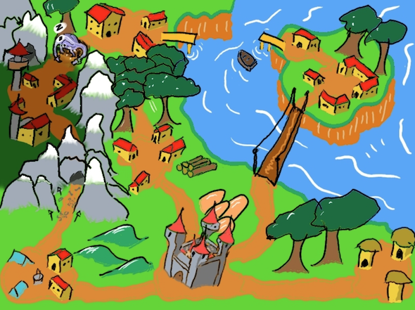
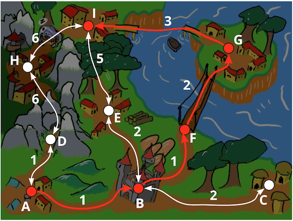
Examining the image above, there are villages, cities, a castle, a bridge, a sleeping dragon, etc. There is too much. To create our graph out of this domain, let's convert all cities and castles into nodes, the paths between them are the edges and the weights are given in accordance to how difficult that path is (it is an arbitrary number, but yet that reflects the scale of difficulty of each). The image below illustrates this process:

In the above image, pay close attention as to why certain edges contain certain weights. The easiest path, from \(A\) to \(B\) for example, gets weight 1. Others, when crossing a bridge or forest, have a bigger weight. The path from the node \(D\) to \(H\), for example, crosses a set of mountains; and the path from \(H\) to \(I\) crosses through the sleeping dragon. Those paths have higher values (6 in this case). After the nodes and edges are created, the rest can be discarded.
By simply rearranging the graph above, we get the one below:
flowchart LR A((A)) B((B)) C((C)) D((D)) E((E)) F((F)) G((G)) H((H)) I((I)) A --1--- B A --1--- D B --2--- C B --2--- E B --1--- F D --6--- H E --5--- I F --2--- G G --3--- I H --6--- I
Let's use this graph through out the A* explanation.
The A* algorithm
To run the A* through a defined graph, the following is necessary:
- The start node
- The end node
- The heuristic function
Looking at the graph created previously, \(A\) is the start node and \(I\) the end node (or the goal). The heuristic function, \(h(n)\) is defined as a mathematical function, domain dependent, that guides the algorithm to the right solution, i.e. the end node. Here "domain dependent" means that the heuristic function will be different for each application.
For our example, the heuristic function is defined as the direct distance of each node to the goal. This function can be, for example, the following table:
| \(n\) | A | B | C | D | E | F | G | H | I |
|---|---|---|---|---|---|---|---|---|---|
| \(h(n)\) | 12 | 7 | 15 | 10 | 5 | 5 | 3 | 6 | 0 |
The heuristic is usually a function defined through a mathematical expression. For easiness, in this case, let's work with a table.
To visualize it, the heuristic function is represented by the red arrows below:
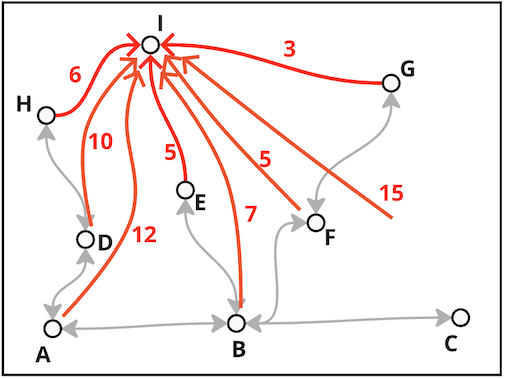
Notice that the value of the heuristics for the nodes \(G\), \(E\) and \(H\) are the same as their distances to \(I\). That is because those nodes share a direction connection with \(I\). Finally, worth pointing out that the heuristics from \(I\) to itself is zero because, of course, that is the node we chose as the end node. Keep in mind that the heuristic changes according to which node is the end node.
Once the cost and the heuristic function are defined, the A* will, for each node, always select the next whose accumulated cost is the lowest. I.e.:
$$ f(n) = g(n) + h(n) $$
Where:
- \(n\) is the node;
- \(g(n)\) is the cost of passing through node \(n\)
- \(h(n)\) is the heuristic of \(n\)
- \(f(n)\) the accumulated cost passing through \(n\)
The algorithm
The algorithm is depicted below:
 1openNodes <- startNode
 2exploredNodes <- empty
 3
 4while openNode is not empty:
 5    node <- openNode.pop()
 6    exploredNodes.append(node)
 7
 8    if node = endNode:
 9        calculatePath
10        break
11
12    for each edge from node:
13        neighborNode <- edge.destination
14
15        if neighborNode not in exploredNodes:
16            neighborNode.parent <- node
17            neighborNode.accumulatedCost <- node.costSoFar + edge.cost
18            neighborNode.passThrough <- node.costSoFar + edge.cost + heuristic(node)
19
20            openNodes.append(neighborNode)
21
22    openNodes.sortNodes()
Right from the start, there are two lists:
openNodes, which contains all the unexplored nodes.exploredNodes, which contains the explored nodes.
The openNodes contain only the startNode at the start. The list exploredNodes is empty. The while loop makes the "magic" happen. It removes the first node from the openNodes and adds it to exploredNodes.
If this node is the endNode, calculate the path and exit. Otherwise, look for the neighboring nodes from node.
For each of those, if the neighborNode is not in the explored list, assign the actual node as its parent, calculate the \(g(\text{neighborNode})\) and add it to openNodes. At the end, sort the openNodes list.
Two things are very important to realize: (i) the explored list avoids cycles (so the algorithm will not revisit a node where it has been before), and (ii) the list of open nodes is sorted at the end of the while loop. This sorting is based on the passThrough value, so the node with the lowest value will be in the position 0.
Going back to the example, the start node is \(A\) and the end node is \(I\).
The node \(A\) is in the openNodes list, and exploredNodes is empty.
flowchart LR A((A)) B((B)) C((C)) D((D)) E((E)) F((F)) G((G)) H((H)) I((I)) A --1--- B A --1--- D B --2--- C B --2--- E B --1--- F D --6--- H E --5--- I F --2--- G G --3--- I H --6--- I style A fill: #99f style I fill: #f99
| OpenNodes | Accumulated Cost | Acc. Cost + Heuristic | Parent |
|---|---|---|---|
| A | 0 | - | - |
| ExploredNodes | Accumulated Cost | Parent |
|---|
The triple notation above means (node, accumulated_cost, passThrough_cost, parent_node). Since \(A\) is the start node, the costs so far are zero and the parent is null.
At the end of the first loop iteration, \(A\) is taken from the list, and its neighbors are checked. Each of them is added to the openList. \(A\) is added to the exploredNodes.
flowchart LR A((A)) B((B)) C((C)) D((D)) E((E)) F((F)) G((G)) H((H)) I((I)) A ab@--1--- B A ad@--1--- D B --2--- C B --2--- E B --1--- F D --6--- H E --5--- I F --2--- G G --3--- I H --6--- I style A fill: #999 style B fill: #9bf style D fill: #9bf style I fill: #f99 ab@{ animate: true; } ad@{ animate: true; } linkStyle 0 stroke: #9bf,stroke-width:3px linkStyle 1 stroke: #9bf,stroke-width:3px
| OpenNodes | Accumulated Cost | Acc. Cost + Heuristic | Parent |
|---|---|---|---|
| B | 1 | 0 + 1 + 7 = 8 | A |
| D | 1 | 0 + 1 + 10 =11 | A |
| ExploredNodes | Accumulated Cost | Parent |
|---|---|---|
| A | 0 | - |
From \(A\), the nodes \(B\) and \(D\) are now open, and the passThrough value of each is cost + heuristic as shown above. The algorithm will then take \(B\) as the next node and will expand from it.
flowchart LR A((A)) B((B)) C((C)) D((D)) E((E)) F((F)) G((G)) H((H)) I((I)) A ab@--1--- B A ad@--1--- D B bc@--2--- C B be@--2--- E B bf@--1--- F D --6--- H E --5--- I F --2--- G G --3--- I H --6--- I style A fill: #999 style B fill: #999 style E fill: #9bf style F fill: #9bf style C fill: #9bf style D fill: #9bf style I fill: #f99 ad@{ animate: true; } bc@{ animate: true; } be@{ animate: true; } bf@{ animate: true; } linkStyle 0 stroke: #999,stroke-width:3px linkStyle 1 stroke: #9bf,stroke-width:3px linkStyle 2 stroke: #9bf,stroke-width:3px linkStyle 3 stroke: #9bf,stroke-width:3px linkStyle 4 stroke: #9bf,stroke-width:3px
| OpenNodes | Accumulated Cost | Acc. Cost + Heuristic | Parent |
|---|---|---|---|
| F | 1 + 1 = 2 | 1 + 1 + 5 = 7 | B |
| E | 1 + 2 = 3 | 1 + 2 + 5 = 8 | B |
| D | 1 | 0 + 1 + 10 =11 | A |
| C | 1 + 2 = 3 | 1 + 2 + 15 = 18 | B |
| ExploredNodes | Accumulated Cost | Parent |
|---|---|---|
| A | 0 | - |
| B | 1 | A |
The cheapest now is \(F\), which is taken from the list and expanded.
flowchart LR A((A)) B((B)) C((C)) D((D)) E((E)) F((F)) G((G)) H((H)) I((I)) A ab@--1--- B A ad@--1--- D B bc@--2--- C B be@--2--- E B bf@--1--- F D --6--- H E ei@--5--- I F fg@--2--- G G --3--- I H --6--- I style A fill: #999 style B fill: #999 style E fill: #9bf style F fill: #999 style C fill: #9bf style D fill: #9bf style G fill: #9bf style I fill: #f99 ad@{ animate: true; } bc@{ animate: true; } be@{ animate: true; } fg@{ animate: true; } linkStyle 0 stroke: #999,stroke-width:3px linkStyle 1 stroke: #9bf,stroke-width:3px linkStyle 2 stroke: #9bf,stroke-width:3px linkStyle 3 stroke: #9bf,stroke-width:3px linkStyle 4 stroke: #999,stroke-width:3px linkStyle 7 stroke: #9bf,stroke-width:3px
| OpenNodes | Accumulated Cost | Acc. Cost + Heuristic | Parent |
|---|---|---|---|
| G | 2 + 2 = 4 | 2 + 2 + 3 = 7 | F |
| E | 1 + 2 = 3 | 1 + 2 + 5 = 8 | B |
| D | 1 | 0 + 1 + 10 = 11 | A |
| C | 1 + 2 = 3 | 1 + 2 + 15 = 18 | B |
| ExploredNodes | Accumulated Cost | Parent |
|---|---|---|
| A | 0 | - |
| B | 1 | A |
| F | 2 | B |
Then, the algorithm will expand the node \(G\), finally leading to having \(I\) in the open list.
flowchart LR A((A)) B((B)) C((C)) D((D)) E((E)) F((F)) G((G)) H((H)) I((I)) A ab@--1--- B A ad@--1--- D B bc@--2--- C B be@--2--- E B bf@--1--- F D --6--- H E ei@--5--- I F fg@--2--- G G gi@--3--- I H --6--- I style A fill: #999 style B fill: #999 style E fill: #9bf style F fill: #999 style C fill: #9bf style D fill: #9bf style G fill: #999 style I fill: #9bf ad@{ animate: true; } bc@{ animate: true; } be@{ animate: true; } gi@{ animate: true; } linkStyle 0 stroke: #999,stroke-width:3px linkStyle 1 stroke: #9bf,stroke-width:3px linkStyle 2 stroke: #9bf,stroke-width:3px linkStyle 3 stroke: #9bf,stroke-width:3px linkStyle 4 stroke: #999,stroke-width:3px linkStyle 7 stroke: #999,stroke-width:3px linkStyle 8 stroke: #9bf,stroke-width:3px
| OpenNodes | Accumulated Cost | Acc. Cost + Heuristic | Parent |
|---|---|---|---|
| I | 4 + 3 = 7 | 4 + 3 + 0 = 7 | G |
| E | 1 + 2 = 3 | 1 + 2 + 5 = 8 | B |
| D | 1 | 0 + 1 + 10 =11 | A |
| C | 1 + 2 = 3 | 1 + 2 + 15 = 18 | B |
| ExploredNodes | Accumulated Cost | Parent |
|---|---|---|
| A | 0 | - |
| B | 1 | A |
| F | 2 | B |
| G | 3 | F |
Finally node \(I\), the end node, is taken. This finalizes the algorithm and the final path is gathered. The path is formed back by simply taking all the parent nodes starting from \(I\), which gives then the path \(A \rightarrow B \rightarrow F \rightarrow G \rightarrow I\) and a total cost of 7.
flowchart LR A((A)) B((B)) C((C)) D((D)) E((E)) F((F)) G((G)) H((H)) I((I)) A ab@--1--- B A ad@--1--- D B bc@--2--- C B be@--2--- E B bf@--1--- F D --6--- H E ei@--5--- I F fg@--2--- G G gi@--3--- I H --6--- I style A fill: #f00 style B fill: #f00 style F fill: #f00 style G fill: #f00 style I fill: #f00 ab@{ animate: true; } bf@{ animate: true; } fg@{ animate: true; } gi@{ animate: true; } linkStyle 0 stroke: #f00,stroke-width:2px linkStyle 4 stroke: #f00,stroke-width:2px linkStyle 7 stroke: #f00,stroke-width:2px linkStyle 8 stroke: #f00,stroke-width:3px
Implementing A*
Any language will do. As usual, I choose to do it in Go. First, define the structs for a Node, an Edge and a Graph. I am also defining a wrappedNode structure, which will contain information such as the accumulated cost and parent node.
 1type Node struct {
 2    Name string
 3}
 4
 5type Edge struct {
 6    Node1 *Node
 7    Node2 *Node
 8    Cost  float32
 9}
10
11type Graph struct {
12    ListNodes []*Node
13    ListEdges []*Edge
14}
15
16// wrapperNode used in the FindBestPath function
17type wrapperNode struct {
18    *Node
19    accumulatedCost float32
20    parent          *wrapperNode
21}
Next are the functions to create each of the above mentioned structures.
 1func CreateNode(name string) *Node {
 2    return &Node{Name: name}
 3}
 4
 5func CreateEdge(node1 *Node, node2 *Node, cost float32) *Edge {
 6    return &Edge{Node1: node1, Node2: node2, Cost: cost}
 7}
 8
 9func CreateGraph(listNodes []*Node, listEdges []*Edge) *Graph {
10    return &Graph{ListNodes: listNodes, ListEdges: listEdges}
11}
12
13func createWrapperNode(node *Node, accCost float32, parentNode *wrapperNode) *wrapperNode {
14    return &wrapperNode{
15        Node:            node,
16        accumulatedCost: accCost,
17        parent:          parentNode,
18    }
19}
As a matter of fact, the information inside wrapperNode could be defined in Node as well. The reason why I kept those separated is because Node is the node per se, while the other carries information that is used only in the A star implementation.
I am also creating a type for the heuristic function, which we will come back later to:
1type HeuristicFunction func(node *Node, goalNode *Node) float32
Our graph object has two methods:
- given a node
n, get all neighbor nodes, and; - given a start and end nodes, and the heuristic function, to calculate the path.
Below is the implementation of these two methods:
 1// getNeighbors will return the neighbor nodes of a given node n
 2// This function will loop through the edges of the graph. For each
 3// edge, if one of the nodes is `n`, add the other to the resulting list.
 4func (g *Graph) getNeighbors(wrapper *wrapperNode) []*wrapperNode {
 5    var nodes []*wrapperNode
 6    for _, edge := range g.ListEdges {
 7        if edge.Node1 == wrapper.Node {
 8            nodes = append(
 9                nodes,
10                createWrapperNode(
11                    edge.Node2,
12                    wrapper.accumulatedCost + edge.Cost,
13                    wrapper
14                )
15            )
16        } else if edge.Node2 == wrapper.Node {
17            nodes = append(
18                nodes,
19                createWrapperNode(
20                    edge.Node1,
21                    wrapper.accumulatedCost + edge.Cost,
22                    wrapper
23                )
24            )
25        }
26    }
27
28    return nodes
29}
30
31// FindBestPath will calculate the best path from start to end nodes using the A*
32// algorithm.
33func (g *Graph) FindBestPath(startNode *Node, endNode *Node, heuristicFunction HeuristicFunction) Result {
34    openList := []*wrapperNode{createWrapperNode(startNode, 0, nil)}
35    var exploredNodes []*Node
36    var wrappedNode *wrapperNode
37
38    // Look for best path
39    for {
40        // Get item from open list
41        wrappedNode = openList[0]
42        // Remove first item from open list
43        openList = openList[1:]
44
45        // Add it to explored nodes
46        exploredNodes = append(exploredNodes, wrappedNode.Node)
47
48        // Check whether this is the end node
49        if wrappedNode.Node == endNode {
50            break
51        }
52
53        // Iterate over the neighbors
54        for _, newWrappedNode := range g.getNeighbors(wrappedNode) {
55            if !isInList(exploredNodes, newWrappedNode.Node) {
56                openList = append(openList, newWrappedNode)
57            }
58        }
59
60        // Sort the openList, keeping cheaper nodes at the beginning.
61        sort.Slice(openList, func(i, j int) bool {
62            node1 := openList[i]
63            node2 := openList[j]
64
65            return node1.accumulatedCost+heuristicFunction(node1.Node, endNode) <
66                node2.accumulatedCost+heuristicFunction(node2.Node, endNode)
67        })
68    }
69
70    // Gather the path
71    var path []*Node
72    for n := wrappedNode; n != nil; n = n.parent {
73        path = append(path, n.Node)
74    }
75    reversedPath := reverse(path)
76
77    return Result{
78        TotalCost:  wrappedNode.accumulatedCost,
79        Path:       reversedPath,
80        PathLength: len(path),
81        StringPath: extractNodeNames(reversedPath),
82    }
83}
Above, the FindBestPath function is the one that will ultimately look for the best path. Following the A* algorithm's logic, it creates the open and explored lists, and in a while loop it:
- removes the first node
- check whether this is the goal
- if not, add the neighbor nodes in the open list
- sort the open list
Notice that when the sort of the open list happens, lines [61, 67], the function takes into account the sum between the accumulated value and the heuristic value.
The value heuristicFunction must match the type HeuristicFunction defined previously. Therefore, when this function is called, a function in that format must be given.
The getNeighbors function (defined on line 4), will cycle through the edges of a given node. When returning the connected nodes, it will also include the accumulated cost to it (lines 12 and 21).
Finally, to call the A* implementation above, it's necessary to define the nodes, the edges and the heuristic function. An example is shown below:
 1func main() {
 2	nodeMap := map[string]*astar.Node{
 3		"A": astar.CreateNode("A"),
 4		"B": astar.CreateNode("B"),
 5		"C": astar.CreateNode("C"),
 6		"D": astar.CreateNode("D"),
 7		"E": astar.CreateNode("E"),
 8		"F": astar.CreateNode("F"),
 9		"G": astar.CreateNode("G"),
10		"H": astar.CreateNode("H"),
11		"I": astar.CreateNode("I"),
12	}
13
14	edgeList := []*astar.Edge{
15		astar.CreateEdge(nodeMap["A"], nodeMap["B"], 1),
16		astar.CreateEdge(nodeMap["A"], nodeMap["D"], 1),
17		astar.CreateEdge(nodeMap["B"], nodeMap["C"], 2),
18		astar.CreateEdge(nodeMap["B"], nodeMap["E"], 2),
19		astar.CreateEdge(nodeMap["B"], nodeMap["F"], 1),
20		astar.CreateEdge(nodeMap["D"], nodeMap["H"], 6),
21		astar.CreateEdge(nodeMap["E"], nodeMap["I"], 5),
22		astar.CreateEdge(nodeMap["F"], nodeMap["G"], 2),
23		astar.CreateEdge(nodeMap["G"], nodeMap["I"], 3),
24		astar.CreateEdge(nodeMap["H"], nodeMap["I"], 6),
25	}
26
27	graph := astar.CreateGraph(
28		convertMapToList(nodeMap), edgeList,
29	)
30
31	heuristicFunction := func(node *astar.Node, goalNode *astar.Node) float32 {
32		switch node {
33		case nodeMap["A"]: return 12
34		case nodeMap["B"]: return 7
35		case nodeMap["C"]: return 15
36		case nodeMap["D"]: return 10
37		case nodeMap["E"]: return 5
38		case nodeMap["F"]: return 5
39		case nodeMap["G"]: return 3
40		case nodeMap["H"]: return 6
41		case nodeMap["I"]: return 0
42		default: panic(fmt.Sprintf("No heuristic for node %s", node.Name))
43		}
44	}
45
46	result := graph.FindBestPath(nodeMap["A"], nodeMap["I"], heuristicFunction)
47
48	fmt.Println("The path is: ", result.StringPath)
49	fmt.Println("The path length is: ", result.PathLength)
50	fmt.Println("The total cost is: ", result.TotalCost)
51
52	fmt.Println("Done")
53}
The execution of this file will give the best path and its cost in the command line:
1$ go run src/main.go
2The path is:  [A B F G I]
3The path length is:  5
4The total cost is:  7
5Done
This is the same path calculated manually above.
Next
This example is a simply introduction to A*. There is much more to it and, of course, nicer and definitely faster implementations. As a next step, I will go into a more applicable and interesting example of the A*.
The code on this page may omit a few details, such as the functions reverse and extractNodeNames. If you are curious, the full code can be seen in this link.
References
https://en.wikipedia.org/wiki/Pathfinding "Wikipedia on Pathfinding" ↩︎
https://en.wikipedia.org/wiki/A*_search_algorithm "Wikipedia on A*" ↩︎
https://ieeexplore.ieee.org/document/4082128 "Peter E. Hart, Niels J. Nilsson, and Bertram Raphael, A Formal Basis for the Heuristic Determination of Minimum Cost Paths" ↩︎
https://aima.cs.berkeley.edu/ "Artificial intelligence a modern approach" ↩︎