See the code here.

For many many years already, sorting is a given in almost any (if not all) programming language. Who never had to sort an array? Sorting by a certain number, a string or even a specific object (provided you know how to compare them) is something very straight forward.

The problem per si is never much about sorting. That can be done in many ways. The actual problem to be solved is how fast sorting can be done. Back in the days, most data collections were relatively small in comparison with nowadays. Not only that, computer power (in both memory and CPU) was definitely not great. Therefore having a faster or smarter way to sort an array would save a lot of computer cycles and, therefore, time - creating a nicer user experience.

That is when Quick Sort comes into place. Created by Tony Hoare in 1959 and published in 1961 [1], the QuickSort can be done in-place and does not require much memory to operate.

Roughly speaking

The algorithm works recursively through partitioning of the array. On the first step, the whole array is one big partition.

The first step of this partitioning is to chose a pivot. Once chosen, every item is compared to it. The goal is to reorder the partition, so that all items to the left of the pivot are smaller, and all the items to the right are bigger. The image below shows a simplified version of this process:

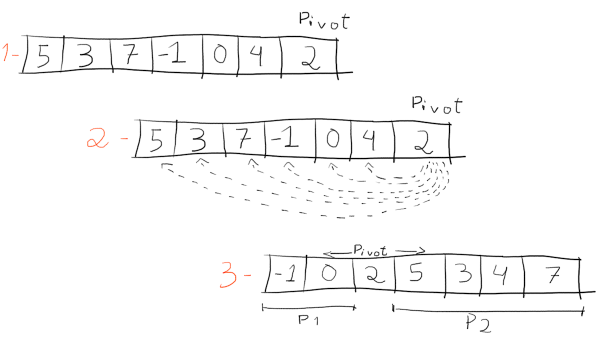
Above, the partitioning was applied to the whole array. At the end, there are two new partitions, P1 and P2. The partitions per se are not ordered, however all items in P1 are smaller than the pivot and all items in P2 are bigger than the pivot. Then, the same process is then applied to each partition recursively.

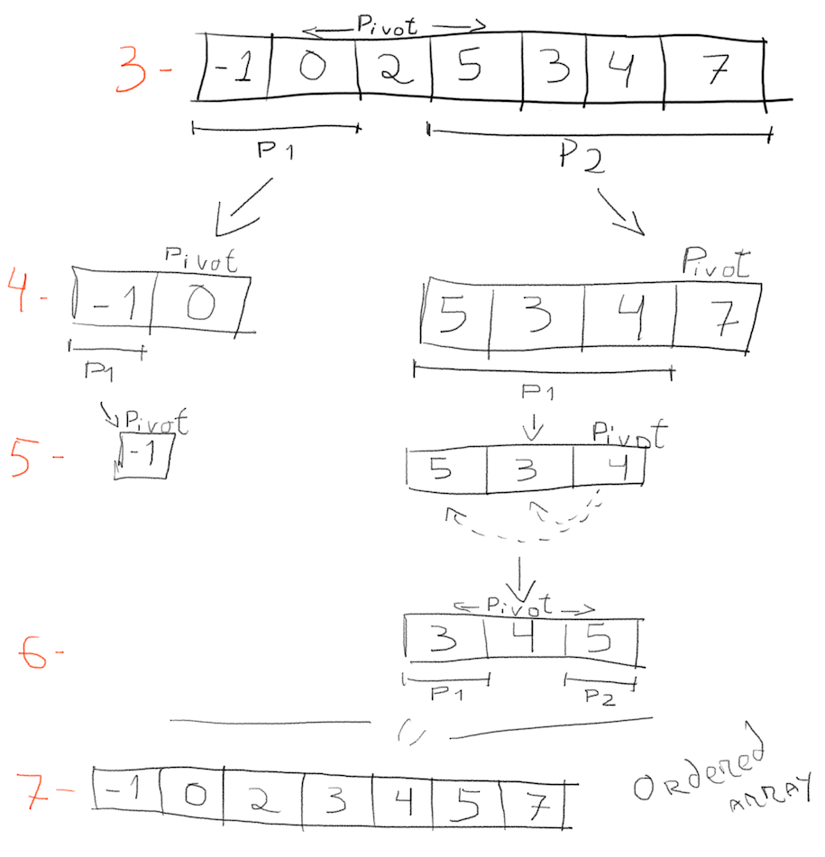
On step 4, the partition [-1, 0] is already ordered, therefore no changes are applied. For the partition [5, 3, 4, 7], all numbers to the left of 7 (the pivot) are already smaller, so again no perceived changes. Step 5, no changes are made to the partition [-1], but the partition [5, 3, 4] is again reordered (the pivot is 4). At 6, numbers to the left of the pivot (4) are smaller and numbers to the right are bigger. Since the remaining partitions contain only one number each, no changes are made. At the very end, step 7, the whole array is ordered.

In code

The code is as straight forward as the description above:

 1func quick(arr []float64, start int, end int) {
 2	if start < end {
 3		pivot_index := partition(arr, start, end)
 4
 5		quick(arr, start, pivot_index)
 6		quick(arr, pivot_index+1, end)
 7	}
 8}
 9
10func QuickSort(arr []float64) []float64 {
11	quick(arr, 0, len(arr))
12}

Above, the function quick calls the function partition on line 3. After it runs, it returns the index of the pivot, which is the split between left and right partitions, as shown in the step 3 of the image 1 above.

Then the quick function is called again recursively for each partition (lines 5 and 6). Finally, the condition on line 2 is what ultimately stops the recursive function. Therefore, most of the quicksort logic relies on the partition function. Below is its implementation.

 1func partition(arr []float64, start int, end int) int {
 2	pivot_index := end - 1
 3	pivot_number := arr[pivot_index]
 4
 5	i := start - 1
 6	for j := start; j < pivot_index; j++ {
 7		if arr[j] < pivot_number {
 8			i++
 9			swap(arr, i, j)
10		}
11	}
12
13	swap(arr, i+1, pivot_index)
14	return i + 1
15}

The pivot is chosen on line 2. In this implementation that is the last number of the partition. Two additional pointers are created: i and j. The first starts outside the partition bounds, i.e. start - 1. The second is placed at the start.

The for loop (lines [6, 12]) moves the pointer j until it meets the index of the pivot. For each number, if that number is lower than the pivot, then it will be swapped with the position pointed by i. At the very end, line 14, the pivot itself is swapped with i.

1func swap(arr []float64, i, j int) {
2	temp := arr[i]
3	arr[i] = arr[j]
4	arr[j] = temp
5}

Example

The partition function is the "core" of the quick sort. Consider the array from the image 1 above: [5, 3, 7, -1, 0, 4, 2]. After running the partition, how does it end up with [-1, 0, 2, 5, 3, 4, 7]?

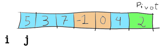
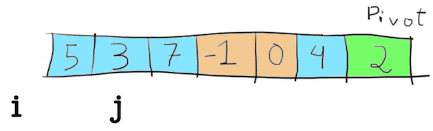
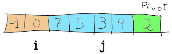
Below is the array, showing i and j (the pointers) at their start positions and the selected pivot, 2. In the image, to make it easier to understand, the pivot is painted green, the numbers that are bigger than the pivot are painted blue and the numbers that are smaller than the pivot are painted orange. This corresponds to the lines [2, 6] of the partition function.

Then comes the for loop, and in each step compared the number pointed by j with the pivot, in our case it makes the comparison 5 < 2, which results in false. Nothing then happens, and j is incremented.

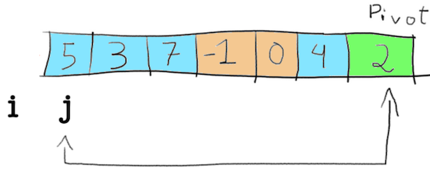
This goes on until j is smaller then the pivot, which happens when j points to -1.

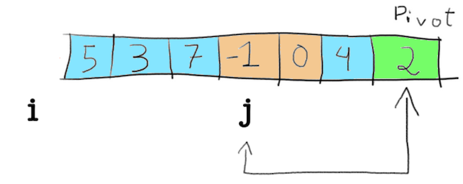
In this moment, i is incremented (line 8 in the partition function), and its number is swapped with j. Therefore, 5 swaps with -1.

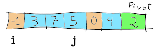
The same happen next, when j points to 0. This value is compared with 2 and, since it is smaller, i is increased by 1 and the values of i and j are swapped.

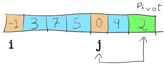
From here, no other number is smaller than 2. Once the for loop finishes, the value pointed by the pointer i + 1 is swapped with the pivot (line 13 in the code).

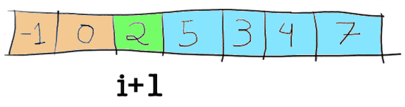
The two partitions P1 and P2, where P1 contains numbers smaller than the pivot and P2 contains numbers bigger than the pivot are here defined. This is the end of the partition function, which will be called again for each of those partitions from here, leading to the breakdown in the image 2 above.

Wrapping up

Quick sort is great and is fast. While I will not dig into its efficiency here, I intend to write about it in the future. The code is also straightforward, though might be challenging if you are seeing it for the first time.

It's quite a classic for whomever had their education in Computer Sciences. As such, I am quite a fan of these well-performing algorithms. It is, sometimes, too bad we don't get to implement these anymore. In other hand, having this already implemented in most computer languages allows professionals to spend their time in more important problems.

If you are a student and are trying to get your head around it, the code of this implementation can be found in this GitHub repository. Feel free to try it out.